
Robert A. Calder, MD, MS; Jayshil J. Patel, MD
WMJ. 2025;124(3):312-316.
W hat is evidence-based medicine? What are the different levels of evidence? Is a testimonial for some treatment considered evidence? How do we know when we have sufficient evidence to draw sound conclusions? For example, is there sufficient evidence to conclude cigarette smoking causes lung cancer? How can we apply evidence to the individual patient? These are the key questions that we will explore in this last part of our series.
WHAT IS “EVIDENCE-BASED MEDICINE?”
By the early 1980s, evidence in medicine was mounting and physicians asked, “How do I sift through the heap of evidence?” Thus, evidence-based medicine pioneer David Sackett introduced the concept of critical appraisal – or the systematic evaluation of clinical research evidence to assess relevance, validity, and applicability to patient care. As it turns out, the term “evidence-based medicine” was an extension of critical appraisal and was used by David Eddy in the late 1980s1 and popularized by Gordon Guyatt and colleagues in a sentinel publication in 1992.2
When the term “evidence-based medicine” came into use, many health care professionals were offended by it, thinking that we have always used evidence in the practice of medicine. In 1980, I (RAC) clearly recall a situation that I thought represented the use of evidence, but, in retrospect, it did not. It was late one Sunday night in the third year of medical school when I was called to a patient’s bedside, and my resident told me to put a nasogastric tube into “Mr. Smith” and irrigate his stomach with iced saline to treat his bleeding gastric ulcer. I recall being happy to do this because I thought that iced saline would cause arterioles to constrict, stopping the bleeding. I also had great confidence in whatever my resident told me to do (“eminence-based” medicine). However, I didn’t realize that no randomized controlled study had ever shown this approach to be beneficial for treating bleeding gastric ulcers. Now, I recognize what I did was because of my understanding of pathophysiology (arterioles bleeding that could constrict in the face of iced saline) and “expert opinion” (my resident’s order). Such a patient would be treated much differently today because of evidence showing that a bacterium, Helicobacter pylori, contributes to ulcer formation and that an antibacterial regimen and gastric acid control are much more effective treatments. It is surprising that much of what we still do in medicine today is based on pathophysiology and expert opinion rooted in tradition, eminence-based medicine, or pathophysiologic rationale rather than high-quality evidence from randomized controlled clinical trials.3
PYRAMID OF EVIDENCE
Evidence in medicine has been likened to a pyramid, with the highest quality evidence at the top and the lowest quality on the bottom. At the top are systematic reviews including one or more meta-analyses of several well-done clinical trials all studying the same outcomes. Below systematic reviews are randomized controlled clinical trials (which vary in quality), followed by prospective epidemiologic studies and retrospective studies (observational studies), then basic research, and finally, expert opinion, case studies, and case reports (clinical experience). Note that “testimonials” from individual users of a treatment are not included in this list.
Randomized controlled trials are the “gold standard” in clinical evidence because when a treatment is randomly and blindly allocated (allocation-concealed) to subjects, and when neither the subjects nor the clinicians know who received which treatment (double blind), the only difference between the groups is the treatment in question. Other factors that could influence the outcome, such as age, sex, race, bias on the part of the investigators, patient expectations, and other confounding factors, are all randomly distributed between the two treatment groups, leaving treatment allocation as the only difference. Furthermore, analyzing all participants in a randomized controlled trial according to their original group assignment—regardless of what occurs after randomization—is known as an intention-to-treat analysis, and it strengthens the validity of the study. When such trials are combined in a valid meta-analysis, statistical power is increased and conclusions are strengthened.
INTERVENTIONAL STUDIES
Broadly speaking, clinical trials can be divided into interventional and observational studies according to whether the investigators are doing something (intervening) or observing, letting “nature take its course.” Interventional studies include randomized controlled studies, non-randomized studies, and non-inferiority studies. Non-randomized studies are sometimes conducted to allow compassionate use of a new treatment. Non-inferiority studies are conducted to determine whether some new treatment is not worse than a standard treatment by more than some certain amount. These studies are conducted more often today when it would be unethical to compare a new treatment with placebo when a well-established treatment is widely available. It is also important to demonstrate that a new treatment, which may have some specific advantages, is not inferior to the standard treatment with respect to important side effects, such as cardiac adverse effects.
OBSERVATIONAL STUDIES
Observational studies frequently are subdivided into case-control, cohort, and cross-sectional studies. Case-control studies begin by identifying “cases,” ie, those who meet some illness definition versus controls who do not meet the definition. Then, various “exposures” are identified to determine whether one or more exposures are more likely to have occurred in those who are cases versus controls. For example, if all the individuals who acquired norovirus on a cruise ship slept in a specific area of the ship and none of the controls did, that would be important evidence to consider when determining the cause of the outbreak. Case-control studies are valuable when studying rare diseases.
Cohort studies begin with “exposed” and “unexposed” groups that are followed forward in time to determine who develops a given disease of interest. Cohort studies can be done prospectively (such as the Framingham study4) or “historically” as when a group of exposed people is identified via health records and then evaluated again at some future date to determine which of the “exposed” and “unexposed” developed disease. Cohort studies are useful when the exposure of interest is rare (eg, asbestos exposure).
Cross-sectional studies assess the prevalence of an exposure—such as COVID vaccination—and an outcome—such as hospitalization—at a single point in time. Because data are collected simultaneously, these studies can determine only the prevalence of exposure among those with and without the outcome. Prevalence reflects both the incidence and duration of a condition (prevalence = incidence × duration). As a result, individuals with longer disease duration are more likely to be captured in cross-sectional studies, since duration significantly influences overall prevalence.
HOW DO WE DECIDE WHICH STATISTICAL TEST TO USE?
Over the past 100 years, many statistical techniques have been developed. How do we decide which of these techniques is most appropriate to evaluate the evidence we plan to collect? It is obviously not appropriate to run every statistical test we can think of and then report the one with the lowest P value—a problem called multiple comparisons that inflates the type I error rate. The evaluation plan for our data should be determined before the first subject is enrolled into a study.
WHAT TYPE OF STUDY ARE YOU PLANNING?
The first consideration is what question you are trying to answer. From there, you can ask what type of study will best answer that question. For example, if you want to know if exposure “x” increases the risk of outcome “y,” then a cohort study design will answer that question. Does your question require you to design a retrospective study? If so, certain statistical measures, such as the odds ratio, will be most appropriate, comparing the odds of disease in groups with various exposures.
Are you planning a prospective study? If so, then the relative risk can be calculated since you will be collecting “incidence” data, and you can compare the incidence of disease in exposed versus unexposed groups.
Do you seek to know if a new intervention improves an outcome compared to existing standard of care interventions? If so, then a randomized controlled clinical trial would provide the strongest evidence to answer the question. Furthermore, if you intend to have “time-to-event” as an outcome measure, such as the time between entry into the study until some “cardiac event” occurs, you will want to consider using the Kaplan-Meier method for estimating survival functions (comparing who does and who does not develop disease) and perhaps comparing the hazard rates for various treatments using Cox Proportional Hazards analysis.5 The hazard rate (discussed in part 2 of this series) reflects how likely a given event is to occur. The higher the hazard rate the lower the survival rate, similar to a teeter totter.6 When the hazard rate is high, the survival rate is low and vice versa. To recap: the Kaplan-Meier method estimates the probability of “survival” (not having an event), and the hazard ratio represents the ratio of the hazard in one group (such as the treatment group) versus another group (such as the control group).
WHAT TYPE OF DATA WILL YOU HAVE?
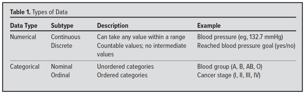 The type of data you plan to collect—regardless of study design—directly influences the statistical tests you can appropriately use. Ask yourself if the data will be numerical or categorical. If numerical, is it continuous (eg, systolic blood pressure measured to 3 decimal places) or discrete (eg, achieving a blood pressure target: yes or no)? If categorical, is it nominal (eg, blood type: A, B, AB, O) or ordinal (eg, cancer stage I to IV)? When working with ordinal data, it is important to choose statistical methods that preserve the natural order of the categories (Table 1).
HOW DO YOU DETERMINE SAMPLE SIZE?
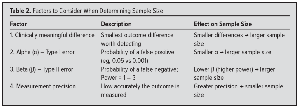 Finally, once you have decided which statistical test to use to evaluate your data, how do you determine an adequate sample size? Although the full methodology is beyond the scope of this discussion, sample size calculations are influenced primarily by 4 factors (Table 2).
First, consider the minimum difference between groups that you consider clinically meaningful. The smaller this difference, the larger the sample size you will need to detect it. Conversely, if you aim to detect a very large difference, a smaller sample may suffice.
Second, consider the alpha level (α)– the probability of a “false alarm” (type I error). The smaller you set alpha, the larger the sample size required, because you’re demanding stronger evidence to declare a result statistically significant.
Third, decide an acceptable beta level (β) – the probability of “missing the boat” (type II error). A smaller beta (eg, 10%, corresponding to 90% power) requires a larger sample size than a higher beta (eg, 20%, or 80% power), because greater power increases your ability to detect a true difference.
Fourth, consider the precision of your outcome measurement. More precise measurements – such as blood pressure recorded to 3 decimal places via arterial line – reduce variability and allow smaller differences to be detected with fewer participants. In contrast, less precise methods – such as using a blood pressure cuff accurate to only +/- 2 mmHg – increase variability and require a larger sample size to detect the same effect.
STATISTICAL PITFALLS
Scientific studies can encounter numerous challenges – from choosing the right participants to correctly analyzing data. This discussion will highlight 2 major concerns.
Bias
Bias is any effect tending to produce results that depart systematically from the true values.7(pp10) Bias must be systematic and not random. If it were random, it would have no overall effect, since one group would be affected as much as any other.
A famous example of bias comes from the work of Abraham Wald.8 Wald, a Hungarian mathematician who escaped the Holocaust and later supported the Allied war effort in the United States, was tasked with improving aircraft survivability. The US Army Air Force collected extensive data on where bullet holes were found on planes that returned safely from bombing runs over the English Channel. After analyzing these data, Wald famously asked a crucial question: Where were the bullet holes on the planes that didn’t return?
Wald concluded that armament should be increased in those areas – because the planes that came back showed where they could sustain damage and still fly home. Stated differently, the planes that made it back to England just demonstrated where an airplane could take a hit and still make it back to base. This is a great example of survivorship bias: focusing only on surviving examples can lead to misleading conclusions. Survivorship bias is just one of many biases that can affect studies–especially observational ones – where biases are not evenly distributed between treatment groups.
Confounding
Confounding is a special type of bias. A confounder is a factor that distorts the apparent magnitude of the effect of a study factor on risk.7(pp21) Such a factor is a determinant of the outcome of interest and is unequally distributed among the exposed and unexposed groups. For example, in 1973, a study associated coffee drinking with myocardial infarction (MI).9 At that time, smokers were more likely to drink coffee than nonsmokers. Since smoking is a cause of MI and because it was unequally distributed in the exposure groups (coffee drinkers and noncoffee drinkers), it gave the illusion that coffee drinking was linked to MI.
In general, confounding is controlled by “stratification,” an analysis technique beyond the scope of this discussion. In essence, the data are divided into “strata” with and without the putative confounder and then reanalyzed to see if the original relationship still exists (eg, coffee drinking and MI).
Association, Correlation and Causation
Association, correlation, and causation have distinct and specific meanings, yet often they are confused or used interchangeably, leading to misunderstanding and misinterpretation of study results.
Association
An association means that events are occurring more often together than expected by chance.7(pp5) This does not imply, however, that one event causes the other.
Correlation
Correlation measures the strength and direction of a linear relationship between two variables.7(pp23) For example, when one variable increases, the other tends to increase as well, forming a pattern that fits a straight line. The correlation coefficient quantifies the linear relationship. However, two variables may be related without a linear pattern. For instance, the velocity of a falling object is related to the height from which it was dropped, but the relationship is nonlinear due to acceleration from gravity. Importantly, correlation does not imply causation. Two things may appear to be related, but that does not imply one causes the other.
Causation
What does it mean to state that something causes something else? What does the term “cause” mean? Perhaps this can best be described with a story.
One of us (RAC) was married several years ago and brought a nice alarm clock into our home, which was in a high-rise condo. Every day at 5:30 AM, the alarm went off. When it went off in the summer months, the sun was rising. It was a nice clock, but the clock did not cause the sun to rise. Nevertheless, there was a strong correlation between the alarm going off and the sun coming up during the summer. Now, suppose in December when the alarm went off, I became upset because the sun was not rising and, as a result, threw the alarm clock out the window (of the high-rise condo), and it fell to the ground and broke into 100 pieces. Did I cause the alarm clock to break by throwing it out the window?
Thinking about this more carefully, was tossing it out the window a necessary cause (that must be present for the outcome to occur)? No, I could have broken the alarm clock any number of creative ways, such as hitting it with a hammer or throwing it against the wall. Therefore, throwing it out the window was not a necessary cause.
Was throwing it out the window a sufficient cause (that alone can produce the outcome)? It was not, since in December in Wisconsin it could have landed in a snowbank and not been damaged at all. Therefore, throwing it out the window was not a sufficient cause for breaking the alarm clock.
Instead, it was a contributory cause (that increases the likelihood of the outcome to occur). I contributed to breaking the clock by throwing it out the window. In medicine, when we say one factor causes another, we usually mean it is a contributory cause – one that plays a meaningful role. Generally, for a cause to warrant study and intervention, it must be significant enough to justify taking action.
“CRITERIA” FOR CAUSATION
How can a contributory cause be determined? In 1965 Sir Austin Bradford Hill presented 9 criteria for determining causation in medicine (eg, smoking and the development of lung cancer):10
- Strength. The stronger an association, the more likely it is to be causal. For example, doctors in England who smoked in the early 1950s were up to 30 times more likely to develop lung cancer.
- Consistency. The same association was observed across all settings.
- Specificity. This criterion implies a one-to-one relationship, a concept rooted in Koch’s postulates. However, it was not fulfilled by smoking and lung cancer – smoking causes multiple diseases, including myocardial infarction, chronic obstructive lung disease, and bladder cancer. Therefore, not every criteria must be met for a factor to be considered a cause.
- Temporality. This indispensable criterion implies the cause precedes the effect. For example, it must be shown that smoking comes before lung cancer.
- Biological gradient (dose-response). The risk of lung cancer increases with the amount of smoking – a strong criterion for causation – because it is unlikely that such a consistent dose-response relationship would occur by chance alone if there were no true cause-and-effect link.
- Plausibility. Is it biologically plausible that inhaling known carcinogens into your alveoli can cause cancer? Yes, it is. However, it is important to recognize that our understanding of many cause-and-effect relationships is incomplete. A lack of current explanation does not rule out a true biological connection.
- Coherence. The cause-and-effect interpretation should align with what we know about the disease. For example, cigarette sales and lung cancer rates have shown a strong association, accounting for the expected time lag in cancer development.
- Experiment. Removing the cause should reduce the effect. Smoking cessation lowers the risk of developing lung cancer.
- Analogy. If experimental animals develop lung cancer when exposed to cigarette smoke, it is reasonable to infer that humans might as well, based on this similarity.
CONCLUSION
Evidence goes beyond pathophysiology and expert opinion, with its strength depending on study design. The results of well-designed randomized controlled trials offer more robust evidence than a case report, case series, or an observational study. The choice of statistical tests should align with the study design and data type. Common challenges include bias and confounding, among others. Most associations are not causal, and Austin Bradford Hill’s criteria provide a useful framework for evaluating causation.
REFERENCES
- Eddy DM. The origins of evidence-based medicine: a personal perspective. Virtual Mentor. 2011;13(1):55-60. doi:10.1001/virtualmentor.2011.13.1.mhst1-1101
- Guyatt G, Cairns J, Churchill D, et al. Evidence-based medicine: a new approach to teaching the practice of medicine. JAMA. 1992;268(17):2420-2425. doi:10.1001/jama.1992.03490170092032
- Ebell MH, Sokol R, Lee A, Simons C, Early J. How good is the evidence to support primary care practice? BMJ Evid Based Med. 2017;22(3):88-92. doi:10.1136/ebmed-2017-110704
- Framingham Heart Study. Accessed August 15, 2025. https://www.framinghamheartstudy.org
- Tolles J, Lewis RJ. Time-to-event analysis. JAMA. 2016;315(10):1046-1047. doi:10.1001/jama.2016.1825
- Kleinbaum DG. Survival Analysis: A Self-Learning Text. Springer; 1996:25,33. doi:10.1007/978-1-4419-6646-9
- Last JM. A Dictionary of Epidemiology. Oxford University Press; 1983:10.
- Wallis WA. The Statistical Research Group, 1942–1945. J Am Stat Assoc. 1980;75(370):320-330
- Jick H, Miettinen OS, Neff RK, Shapiro S, Heinonen OP, Slone D. Coffee and myocardial infarction. N Engl J Med. 1973;289(2):63-67. doi:10.1056/NEJM197307122890203
- Hill AB. The environment and disease: association or causation? Proc R Soc Med. 1965;58(5):295-300. doi:10.1177/003591576505800503
PART 5: DESCRIPTIVE STATISTICS PRACTICE QUESTIONS AND ANSWERS
-
What is the mean of the following numbers: 1, 2, 3, 4, 7, 8? The sum of these 6 numbers (1, 2, 3, 4, 7, 8) is 25. The mean is 25/6 = 4.167
-
What is the median of the following numbers: 2, 5, 9, 16, 22, 25? The median of these numbers (2, 5, 9, 16, 22, 25) is the average of the middle 2 numbers (9 and 16). Therefore, the median is (9 + 16)/2 = 12.5
-
If the mean systolic blood pressure of all patients in your practice is 130 mmHg and the standard deviation is 6 mmHg, what percent of your practice would you expect to have systolic pressures above 142 mmHg assuming the systolic pressures follow a normal distribution? Since the population standard deviation is 6 mmHg, and the mean is 130, 142 is 2 standard deviations above the mean. In a normal distribution, 95% of values are within 2 standard deviations of the mean (2.5% above and 2.5% below 2 standard deviations).
-
Suppose you record the blood pressures of the next 9 patients in your office and calculate the mean systolic pressure of that sample to be 134 mmHg. Would that mean surprise you? What is the standard error of the mean for this random sample of 9? For a sample size of 9, the standard error of the mean (SEM) is the population standard deviation (6) divided by the square root of the sample size (square root of 9 is 3). Therefore, the SEM is 6/3 = 2. Since 134 is 2 standard deviations above the mean, it would not be terribly surprising (P = 0.05).
-
What would the standard error of the mean be for a random sample of 36 of your patients? For a sample of 36, the SEM would be 6/(square root of 36). Therefore, the SEM for a random sample of 36 would be 1.0. Note that to cut the standard error in half (from 2 to 1), the sample size must increase 4 times (from 9 to 36).