
Robert A. Calder, MD, MS; Jayshil J. Patel, MD
WMJ. 2025;124(1)74-77.
Probability is a key concept when interpreting diagnostic tests and explaining data to patients.1 Stephen Jay Gould (1941-2002) stated, “Misunderstanding of probability may be the greatest of all general impediments to scientific literacy.” Therefore, we think that it is important to gain a deeper understanding of probability and how it relates to statistics. In this installment of the Statistical Thinking in Medicine series, we aim to (1) define and interpret probability, (2) describe independent events and the relationship between probability and statistics, (3) define and exemplify the central limit theorem, (4) outline normal and t-distributions, and (5) introduce the regression to the mean.
DEFINITION OF PROBABILITY
Probability is the extent to which an event is likely to occur and has its origins in games of chance. As we understand it today, the modern concepts of probability were first described in a series of letters in the mid-17th century between Pascal and Fermat.2 In essence, for equally likely events, they defined the classical approach to probability by stating that if an event can occur in “k” different ways out of a total of “n” attempts, the probability of it occurring is k/n.3 The main problem with this definition is that “equally likely” is vague. What does “equally likely” mean?
To address this question, the “frequency approach” to probability was developed. In that approach, if an event occurs k times out of n possible occurrences, where n is a large number, the probability is k/n as with the classical approach described above.4 However, the term large number is vague and now the question is: what is a large number?
To address these issues and to put probability on a firmer mathematical footing, Andrey Kolmogorov proposed three axioms for probability in 1933.4 An “axiom” is a statement accepted without proof. The three axioms have been described as a “wish list”5 to define probability functions. That is, if a function satisfies the wish list, it is a probability function. Recall that in mathematics, a function is a mathematical operation in which an “input” is provided, and for each input, a unique “output” is returned. In probability, the input is an “event” eg, heads or tails, and the output is a number between zero and 1. Kolmogorov’s axioms usually are expressed as follows:
- The probability of an event (among all events in some outcome space) is ≥ 0, that is, it is non-negative. There are no negative probabilities.
- The sum of the probabilities of all mutually exclusive events in some sample space is 1. Mutually exclusive events cannot occur at the same time, eg, the flip of a coin is either heads or tails, it has to be one or the other, they cannot both occur at the same time.
- If two events are mutually exclusive, the probability that either occurs is the sum of the two probabilities. This is referred to as the “additive rule.”
PROBABILITY INTERPRETATIONS
Although Kolmogorov’s axioms put probability on a firmer mathematical footing (as Euclid’s axioms did for geometry), the interpretation of this number between zero and 1 is still unclear. As discussed in part 2 of our series, the two most common interpretations of probability are the “frequentist” and the Bayesian interpretations.4 The frequentist interpretation is that probability is a long-run frequency of the occurrence of an event over a large number of repetitions of an experiment performed under similar conditions. The Bayesian view is that probability is a degree of belief about an event, which can then be modified with additional data.
As we discussed in part 3, the Bayesian approach to probability is very useful when evaluating diagnostic tests. However, the Bayesian approach to data analysis presents mathematical challenges beyond the scope of this article. In essence, one either has to find mathematical functions that are “updateable” with additional data (of which the beta distribution is one)6 or use other methods well beyond this brief summary and our expertise. A principal reason for the frequentist approach to data analysis, which is by far the most common approach today, is that no assumptions are required regarding the “prior probability” of some event. The frequentist approach is also computationally more straightforward, in general. Bland provides examples and an accessible introduction to this topic.7
 INDEPENDENT EVENTS
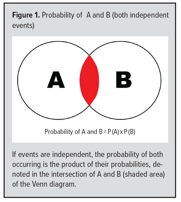
Kolmogorov’s axioms describe single events. If two events are of interest, they are considered “independent” if the probability that they both occur is the product of their independent probabilities.4 For example, suppose the probability of a positive diagnostic test is 0.5 and that tests done on separate days are independent. Then the probability of positive tests two days in a row is: 0.5 x 0.5 = 0.25. Venn diagrams are very helpful for visualizing such intersection probabilities as shown in Figure 1. The product of independent events is often called the “multiplicative rule.” Again, this rule only applies to independent events. Another way to describe independence is when the occurrence of one event provides no information whatsoever about the occurrence of another (independent) event.
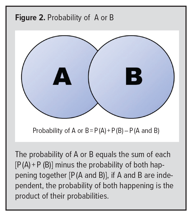 In medicine, we frequently are interested in the “union” of two events. For example, as above, if the probability of a positive test is 0.5 and the test is done two days in a row, what is the probability that the test is positive on either (or both) days? Again, Venn diagrams are very helpful. The probability of at least one positive test is the probability of being positive on day 1 plus the probability of being positive on day 2, MINUS the probability of being positive on both days (to avoid counting this twice): 0.5 + 0.5 – 0.25 = 0.75. This is easy to visualize in Figure 2. An alternative way to calculate such probabilities is to calculate the “complement” of a positive test on one or the other day, ie, the probability of being negative on both days. That probability is 0.5 x 0.5 = 0.25. This complement is then subtracted from 1 to arrive at the probability of being positive at least once (ie, 1 minus the probability of being negative on both days means that the test was positive on at least one day).
A large number of problems in probability can be solved by using the additive and/or the multiplicative rules as appropriate.
 THE RELATIONSHIP BETWEEN PROBABILITY AND STATISTICS
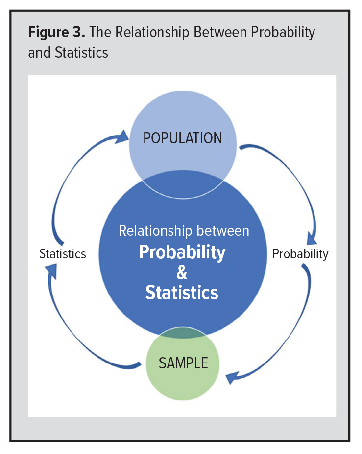
We turn now to the relationship between probability and statistics (Figure 3).8 Probability takes us from some population to any given sample. For example, given a “population” of red and white marbles, probability theory can tell us the exact probability of any given sample (eg, 5 white and 2 red marbles) whenever we randomly sample from the population (either with or without replacement).
Moreover, a random sample allows us to infer about the true nature of a population. For example, if as above, our random sample contains a certain proportion of red marbles, statistics allows us to estimate the range within which the true proportion of red marbles is likely to be with any desired level of confidence. As the sample size increases, the precision of the estimate also increases.
THE CENTRAL LIMIT THEOREM AND NORMAL DISTRIBUTION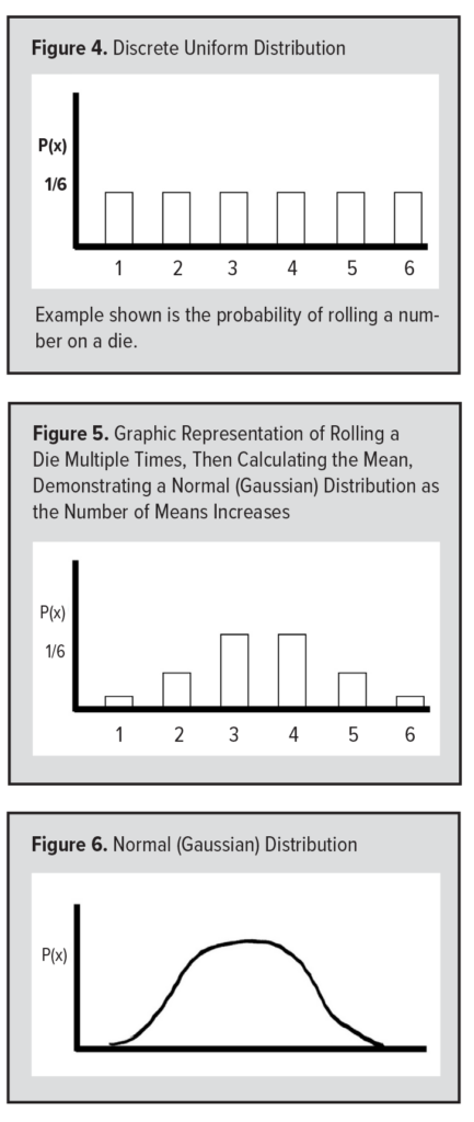
The reason we are able to infer about a population from a random sample is because of the central limit theorem (CLT). In essence, this theorem states that if some given population distribution has a finite mean and variance (to be defined in the next article), the means of random samples from that distribution become normally distributed as the number of samples becomes large.5 What does this mean? This deceptively simple principle allows us to learn about a population from a random sample. In a very real sense, without the CLT, science would not be possible!
A nice way to demonstrate the CLT is to roll a die several times and calculate the average of these rolls. For each number on the die, the probability is 1/6. The distribution for the values of the die is a “discrete uniform” distribution (Figure 4). This discrete uniform distribution, however, changes to a normal distribution if we graph the means of many rolls of the die. For example, if I roll a die five times, the average of these rolls is usually about 3 or 4 (when rounding to the nearest whole number), occasionally 2 or 5, and, very rarely, 1 or 6. If we graph the mean values of many rolls of a die, that graph will begin to take the shape of a normal (or Gaussian) distribution as the number of means increases (Figure 5). This is why the normal distribution is the most important distribution in statistics (Figure 6). Yes, many physical parameters are normally distributed in and of themselves, such as height and weight, but the means of ANY physiological parameter will have a normal distribution. 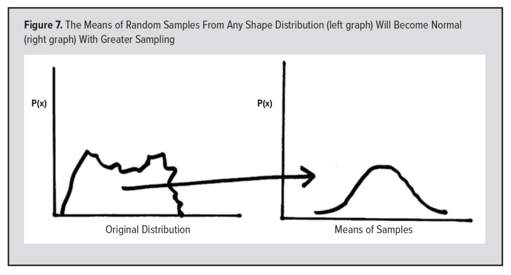 Therefore, the means of random samples from any shape distribution will become normal as the number of samples becomes large (Figure 7). Thus, the CLT allows us to learn about a population from a random sample.
T-DISTRIBUTION
The smaller the sample, the less likely it will be to closely follow the normal distribution. That is why W.S. Gosset, who wrote under the pseudonym “Student” developed the t-distribution. (He was working for the Guiness Brewing Company at the time and found the need to analyze small samples of yeast and related components of beer).9 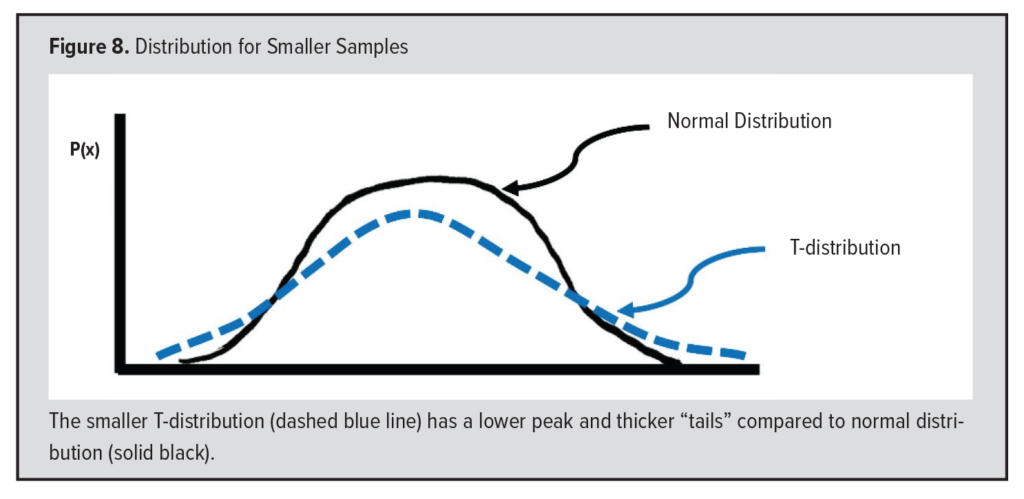 The t-distribution is very similar to the normal distribution, except that it has thicker “tails” and a lower peak (Figure 8).5 Unusual values can easily skew a small distribution, and when the sample size is under about 30, most statisticians prefer using the t-distribution since it accounts for this distortion seen in small samples.
REGRESSION TO MEAN
Closely related to the CLT is the concept of “regression to the mean,” first described by Sir Francis Galton.10 In essence, results become more “average” over time. For example, in 1961, Roger Maris broke Babe Ruth’s home run record by hitting 61 home runs. However, in 1962, Maris hit 33 home runs, a number much more typical for him. He had one exceptional year and that was followed by a more average year. This is a great example of regression to the mean. Other examples are that tall parents are likely to have children more average in height. One high blood pressure reading is likely to be followed by lower, more average, readings. Also, one low test score is likely to be followed by higher, more typical scores. Regression to the mean explains many surprising occurrences.
SUMMARY
In summary, probability is a number between zero and 1 that satisfies three axioms. If events are independent, the probability of both occurring is the product of their probabilities (multiplicative rule). If events are mutually exclusive, the probability that at least one occurs is their sum (additive rule). Probability takes us from a population to a sample, and statistics allows us to infer about a population from a random sample. The CLT and the normal distribution are two important links in the chain connecting a random sample and a population. Finally, regression to the mean answers many probability curiosities.
In part 5 of this series, we will use these principles of probability to determine whether something is unusual. Is an individual value unusual? Is the mean of some group unusual? Is the difference between two or more means unusual? In order to do this, we must have ways to define the “average” and to quantify variation. However, before turning to that topic, you may want to test your ability to put probability concepts to work by thinking about the questions below. (Answers will be provided in part 5.)
PROBABILITY PRACTICE QUESTIONS
- When rolling a die, what is the probability of rolling a 1 or a 2?
- If the probability that a laboratory test is positive is 40%, assuming test results on different days are independent, what is the probability of at least one positive test when testing is done on two separate days?
- As with the conditions in question 2, what is the probability that at least one test is positive if tests are done 5 days in a row?
- To make a diagnosis, suppose you order 20 independent laboratory tests, each of which is “normal” in 95% of people. What is the probability that at least 1 test is abnormal?
- How many ways are there to shuffle a standard deck of 52 cards?
REFERENCES
- Calder RA, Gavinski K, Patel JJ. Statistical Thinking Part 3: Interpreting Diagnostic Tests with Probabilistic Thinking. WMJ. 2024;123(5): 407-411.
- Stigler SM. The History of Statistics: The Measurement of Uncertainty Before 1900. Belknap Press; 1986:4.
- Jaynes ET. Probability Theory: the Logic of Science. Cambridge University Press; 2003:20,43.
- Blitzstein JK, Hwang J. Introduction to Probability. 2nd ed. CRC Press; 2019:21-23,63.
- Daniel WW. Biostatistics: A Foundation For Analysis In The Health Sciences. 3rd ed. John Wiley & Sons; 1983:38-39,102,136-143.
- Kurt W. Bayesian Statistics The Fun Way Understanding Statistics and Probability with Star Wars, LEGO, and Rubber Ducks. No Starch Press; 2019: 45-55.
- Bland M. An Introduction to Medical Statistics. 4th ed. Oxford University Press; 2015:357-366.
- Devore JL. Probability and Statistics for Engineering and The Sciences. 9th ed. Cengage Learning; 2015:6.
- Pearson ES. ‘Student’ A Statistical Biography of William Sealy Gosset. Plackett RL, Barnard GA eds. Clarendon Press; 1990.
- Gail MH, Benichou J, Armitage P, eds, in: Encyclopedia of Epidemiologic Methods. Wiley; 2000:110.